Building Gaussian Naive Bayes Classifier in Python
In this post, we are going to implement the Naive Bayes classifier in Python using my favorite machine learning library scikit-learn. Next, we are going to use the trained Naive Bayes (supervised classification), model to predict the Census Income.
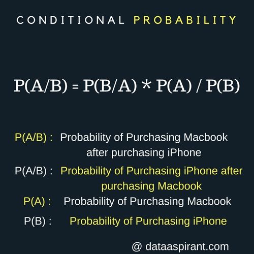
As we discussed the Bayes theorem in naive Bayes classifier post. We hope you know the basics of the Bayes theorem. If not let’s quickly look at the basics of Bayes theorem once.
Bayes’ theorem is based on conditional probability. The conditional probability helps us calculating the probability that something will happen, given that something else has already happened. Not getting let’s understand with few examples.
Conditional Probability Examples
Below are the few examples helps to clearly understand the definition of conditional probability.
- Purchasing mac book when you already purchased the iPhone.
- Having a refreshing drink when you are in the movie theater.
- Buying peanuts when you brought a chilled soft drink.
Conditional Probability Example
Using the Bayes theorem the naive Bayes classifier works. The naive Bayes classifier assumes all the features are independent to each other. Even if the features depend on each other or upon the existence of the other features. Naive Bayes classifier considers all of these properties to independently contribute to the probability that the user buys the MacBook.
To learn the key concepts related to Naive Bayes. You can read our article on Introduction to Naive Bayes. This will help you understand the core concepts related to Naive Bayes.
In the introduction to Naive Bayes post, we discussed three popular Naive Bayes algorithms:
- Gaussian Naive Bayes,
- Multinomial Naive Bayes.
- Bernoulli Naive Bayes.
As a continues to the Naive Bayes algorithm article. Now we are going to implement Gaussian Naive Bayes on a “Census Income” dataset.
Gaussian Naive Bayes
A Gaussian Naive Bayes algorithm is a special type of NB algorithm. It’s specifically used when the features have continuous values. It’s also assumed that all the features are following a gaussian distribution i.e, normal distribution.
Census Income Dataset
Census Income dataset is to predict whether the income of a person >$50K/yr (greater than $50K/yr) or <=$50K/yr. The data was collected by Barry Becker from 1994 Census dataset.
This dataset was contributed to UCI repository, and It’s openly available at this link. The dataset consists of 15 columns of a mix of discrete as well as continuous data.
| Variable Name | Variable Range | |
| 1. | age | [17 – 90] |
| 2. | workclass | [‘State-gov’, ‘Self-emp-not-inc’, ‘Private’, ‘Federal-gov’, ‘Local-gov’, ‘Self-emp-inc’, ‘Without-pay’, ‘Never-worked’] |
| 3. | fnlwgt | [77516- 257302] |
| 4. | education |
[‘Bachelors’, ‘HS-grad’, ’11th’, ‘Masters’, ‘9th’, ‘Some-college’, ‘Assoc-acdm’, ‘Assoc-voc’, ‘7th-8th’, ‘Doctorate’, ‘Prof-school’, ‘5th-6th’, ’10th’, ‘1st-4th’, ‘Preschool’, ’12th’] |
| 5. | education_num | [1 – 16] |
| 6. | marital_status |
[‘Never-married’, ‘Married-civ-spouse’, ‘Divorced’, ‘Married-spouse-absent’, ‘Separated’, ‘Married-AF-spouse’, ‘Widowed’] |
| 7. | occupation |
[‘Adm-clerical’, ‘Exec-managerial’, ‘Handlers-cleaners’, ‘Prof-specialty’, ‘Other-service’, ‘Sales’, ‘Craft-repair’, ‘Transport-moving’, ‘Farming-fishing’, ‘Machine-op-inspct’, ‘Tech-support’, ‘Protective-serv’, ‘Armed-Forces’, ‘Priv-house-serv’] |
| 8. | relationship |
[‘Not-in-family’, ‘Husband’, ‘Wife’, ‘Own-child’, ‘Unmarried’, ‘Other-relative’] |
| 9. | race |
[‘White’, ‘Black’, ‘Asian-Pac-Islander’, ‘Amer-Indian-Eskimo’, ‘Other’] |
| 10. | sex |
[‘Male’, ‘Female’] |
| 11. | capital_gain | [0 – 99999] |
| 12. | capital_loss | [0 – 4356] |
| 13. | hours_per_week | [1 – 99] |
| 14. | native_country |
[‘United-States’, ‘Cuba’, ‘Jamaica’, ‘India’, ‘Mexico’, ‘South’, ‘Puerto-Rico’, ‘Honduras’, ‘England’, ‘Canada’, ‘Germany’, ‘Iran’, ‘Philippines’, ‘Italy’, ‘Poland’, ‘Columbia’, ‘Cambodia’, ‘Thailand’, ‘Ecuador’, ‘Laos’, ‘Taiwan’, ‘Haiti’, ‘Portugal’, ‘Dominican-Republic’, ‘El-Salvador’, ‘France’, ‘Guatemala’, ‘China’, ‘Japan’, ‘Yugoslavia’, ‘Peru’, ‘Outlying-US(Guam-USVI-etc)’, ‘Scotland’, ‘Trinadad&Tobago’, ‘Greece’, ‘Nicaragua’, ‘Vietnam’, ‘Hong’, ‘Ireland’, ‘Hungary’, ‘Holand-Netherlands’] |
| 15. | income |
[‘<=50K’, ‘>50K’] |
The final target variable consists of two values: ‘<=50K” & ‘>50K’.
Implementation of Gaussian NB on Census Income dataset
Importing Python Machine Learning Libraries
We need to import pandas, numpy and sklearn libraries. From sklearn, we need to import preprocessing modules like Imputer. The Imputer package helps to impute the missing values.
If you are not setup the python machine learning libraries setup. You can first complete it to run the codes in this articles.
|
1
2
3
4
5
6
7
8
9
10
11
12
|
# Required Python Machine learning Packages
import pandas as pd
import numpy as np
# For preprocessing the data
from sklearn.preprocessing import Imputer
from sklearn import preprocessing
# To split the dataset into train and test datasets
from sklearn.cross_validation import train_test_split
# To model the Gaussian Navie Bayes classifier
from sklearn.naive_bayes import GaussianNB
# To calculate the accuracy score of the model
from sklearn.metrics import accuracy_score
|
The train_test_split module is for splitting the dataset into training and testing set. The accuracy_score module will be used for calculating the accuracy of our Gaussian Naive Bayes algorithm.
Data Import
For importing the census data, we are using pandas read_csv() method. This method is a very simple and fast method for importing data.
We are passing four parameters. The ‘adult.data’ parameter is the file name. The header parameter is for giving details to pandas that whether the first row of data consists of headers or not. In our dataset, there is no header. So, we are passing None.
The delimiter parameter is for giving the information the delimiter that is separating the data. Here, we are using ‘ *, *’ delimiter. This delimiter is to show delete the spaces before and after the data values. This is very helpful when there is inconsistency in spaces used with data values.
|
1
2
|
adult_df = pd.read_csv(‘adult.data’,
header = None, delimiter=‘ *, *’, engine=‘python’)
|
Let’s add headers to our dataframe. The below code snippet can be used to perform this task.
|
1
2
3
4
|
adult_df.columns = [‘age’, ‘workclass’, ‘fnlwgt’, ‘education’, ‘education_num’,
‘marital_status’, ‘occupation’, ‘relationship’,
‘race’, ‘sex’, ‘capital_gain’, ‘capital_loss’,
‘hours_per_week’, ‘native_country’, ‘income’]
|
Handling Missing Data
Let’s try to test whether there is any null value in our dataset or not. We can do this using isnull()method.
|
1
|
adult_df.isnull().sum()
|
Script Output
|
1
2
3
4
5
6
7
8
9
10
11
12
13
14
15
16
|
age 0
workclass 0
fnlwgt 0
education 0
education_num 0
marital_status 0
occupation 0
relationship 0
race 0
sex 0
capital_gain 0
capital_loss 0
hours_per_week 0
native_country 0
income 0
dtype: int64
|
The above output shows that there is no “null” value in our dataset.
Let’s try to test whether any categorical attribute contains a “?” in it or not. At times there exists “?” or ” ” in place of missing values. Using the below code snippet we are going to test whether our adult_df data frame consists of categorical variables with values as “?”.
|
1
2
3
4
5
|
for value in [‘workclass’, ‘education’,
‘marital_status’, ‘occupation’,
‘relationship’,‘race’, ‘sex’,
‘native_country’, ‘income’]:
print value,“:”, sum(adult_df[value] == ‘?’)
|
Script Output
|
1
2
3
4
5
6
7
8
9
|
workclass : 1836
education : 0
marital_status : 0
occupation : 1843
relationship : 0
race : 0
sex : 0
native_country : 583
income : 0
|
The output of the above code snippet shows that there are 1836 missing values in workclassattribute. 1843 missing values in occupation attribute and 583 values in native_country attribute.
Data preprocessing
For preprocessing, we are going to make a duplicate copy of our original dataframe.We are duplicating adult_df to adult_df_rev dataframe.
|
1
|
adult_df_rev = adult_df
|
As we want to perform some imputation for missing values. Before doing that, we need some summary statistics of our dataframe. For this, we can use describe() method. It can be used to generate various summary statistics, excluding NaN values.
We are passing an “include” parameter with value as “all”, this is used to specify that. we want summary statistics of all the attributes.
|
1
|
adult_df_rev.describe(include= ‘all’)
|
Data Imputation Step
|
1
2
3
4
5
6
|
for value in [‘workclass’, ‘education’,
‘marital_status’, ‘occupation’,
‘relationship’,‘race’, ‘sex’,
‘native_country’, ‘income’]:
adult_df_rev[value].replace([‘?’], [adult_df_rev.describe(include=‘all’)[value][2]],
inplace=‘True’)
|
We have performed data imputation step. 🙂
You can check changes in dataframe by printing adult_df_rev
One-Hot Encoder
|
1
2
3
4
5
6
7
8
9
|
le = preprocessing.LabelEncoder()
workclass_cat = le.fit_transform(adult_df.workclass)
education_cat = le.fit_transform(adult_df.education)
marital_cat = le.fit_transform(adult_df.marital_status)
occupation_cat = le.fit_transform(adult_df.occupation)
relationship_cat = le.fit_transform(adult_df.relationship)
race_cat = le.fit_transform(adult_df.race)
sex_cat = le.fit_transform(adult_df.sex)
native_country_cat = le.fit_transform(adult_df.native_country)
|
|
1
2
3
4
5
6
7
8
9
|
#initialize the encoded categorical columns
adult_df_rev[‘workclass_cat’] = workclass_cat
adult_df_rev[‘education_cat’] = education_cat
adult_df_rev[‘marital_cat’] = marital_cat
adult_df_rev[‘occupation_cat’] = occupation_cat
adult_df_rev[‘relationship_cat’] = relationship_cat
adult_df_rev[‘race_cat’] = race_cat
adult_df_rev[‘sex_cat’] = sex_cat
adult_df_rev[‘native_country_cat’] = native_country_cat
|
|
1
2
3
4
5
|
#drop the old categorical columns from dataframe
dummy_fields = [‘workclass’, ‘education’, ‘marital_status’,
‘occupation’, ‘relationship’, ‘race’,
‘sex’, ‘native_country’]
adult_df_rev = adult_df_rev.drop(dummy_fields, axis = 1)
|
Using the above code snippets, we have created multiple categorical columns like “marital_cat”, “race_cat” etc. You can see the top 6 lines of the dataframe using adult_df_rev.head()By printing the adult_df_rev.head() result. You will be able to see that all the columns should be reindexed. They are not in proper order. For reindexing the columns, you can use the code snippet provided below:
|
1
2
3
4
5
6
7
|
adult_df_rev = adult_df_rev.reindex_axis([‘age’, ‘workclass_cat’, ‘fnlwgt’, ‘education_cat’,
‘education_num’, ‘marital_cat’, ‘occupation_cat’,
‘relationship_cat’, ‘race_cat’, ‘sex_cat’, ‘capital_gain’,
‘capital_loss’, ‘hours_per_week’, ‘native_country_cat’,
‘income’], axis= 1)
adult_df_rev.head(1)
|
The output to the above code snippet will show you that all the columns are reindexed properly. I have passed the list of column names as a parameter and axis=1 for reindexing the columns.
Standardization of Data
All the data values of our dataframe are numeric. Now, we need to convert them on a single scale. We can standardize the values. We can use the below formula for standardization.
} {\sigma(x)}")
|
1
2
3
4
5
6
7
8
9
10
|
num_features = [‘age’, ‘workclass_cat’, ‘fnlwgt’, ‘education_cat’, ‘education_num’,
‘marital_cat’, ‘occupation_cat’, ‘relationship_cat’, ‘race_cat’,
‘sex_cat’, ‘capital_gain’, ‘capital_loss’, ‘hours_per_week’,
‘native_country_cat’]
scaled_features = {}
for each in num_features:
mean, std = adult_df_rev[each].mean(), adult_df_rev[each].std()
scaled_features[each] = [mean, std]
adult_df_rev.loc[:, each] = (adult_df_rev[each] – mean)/std
|
We have converted our data values into standardized values. You can print and check the output of dataframe.
Data Slicing
Let’s split the data into training and test set. We can easily perform this step using sklearn’s train_test_split() method.
|
1
2
3
4
|
features = adult_df_rev.values[:,:14]
target = adult_df_rev.values[:,14]
features_train, features_test, target_train, target_test = train_test_split(features,
target, test_size = 0.33, random_state = 10)
|
Using above code snippet, we have divided the data into features and target set. The feature set consists of 14 columns i.e, predictor variables and target set consists of 1 column with class values.
The features_train & target_train consists of training data and the features_test & target_testconsists of testing data.
Gaussian Naive Bayes Implementation
After completing the data preprocessing. it’s time to implement machine learning algorithm on it. We are going to use sklearn’s GaussianNB module.
|
1
2
3
|
clf = GaussianNB()
clf.fit(features_train, target_train)
target_pred = clf.predict(features_test)
|
We have built a GaussianNB classifier. The classifier is trained using training data. We can use fit()method for training it. After building a classifier, our model is ready to make predictions. We can use predict() method with test set features as its parameters.
Accuracy of our Gaussian Naive Bayes model
It’s time to test the quality of our model. We have made some predictions. Let’s compare the model’s prediction with actual target values for the test set. By following this method, we are going to calculate the accuracy of our model.
|
1
|
accuracy_score(target_test, target_pred, normalize = True)
|
Script Output
|
1
|
0.80141447980643965
|
Awesome! Our model is giving an accuracy of 80%. This is not bad with a simple implementation. You can create random test datasets and test the model to get know how well the trained Gaussian Naive Bayes model is performing.
We can save the trained scikit-learn model with Python pickle. You can check out how to save the trained scikit-learn model with Python Pickle.
Source: http://dataaspirant.com/2017/02/20/gaussian-naive-bayes-classifier-implementation-python/


